Sweet spots for analysis

Robustness, fragility, and other analogies between optimization and control.

This is a live blog of Lecture 1 of my graduate seminar “Feedback, Learning, and Adaptation.” There are some equations below, but I tried to keep them to a minimum and stick them at the end.

Interconnection warps systems in surprising ways. Even in the simplest settings, two components in feedback behave differently than when disconnected. In the example from the last post, there was no single component that achieved the task of reliable amplification. We connected an unreliable, underspecified large amplifier to an accurate attenuator, yielding a balance between accuracy and amplification. Feedback created an unexpectedly robust operating condition.

The interconnection is also fragile in interesting ways. While the amplifier can vary widely and unpredictably, the attenuator must be precisely tuned to achieve the desired gain. One of the components needs to be accurate when the other is inaccurate. Similarly, the model here assumes that the system immediately reaches its fixed point when an input is applied. In reality, these components are comprised of circuitry with temporal dynamics. You can convince yourself by an experiment (or you can just write out the math) that if there is any delay in the trip from the amplifier’s input to the attenuator’s output, the whole system will blow up. The accurate component needs to be faster than the inaccurate one. And I didn’t model these dynamics at all in the last post. A recurring theme here—one drilled into my head by a quarter century of conversations with John Doyle—is that any designed interconnected system that seems to exhibit impressive robustness has some fragility hiding in plain sight.

One worry in the comments on Monday’s post noted that this sort of analysis doesn’t work for nonlinear systems. In this class, my hope is to explain why that’s not quite true. Let me relate nonlinear control to something that might be more familiar: nonlinear optimization. In unconstrained optimization, you first study minimizing quadratic functions and then perhaps move on to general optimization. The insights from quadratics provide practical heuristics for dealing with more general optimization. For example, the conjugate gradient method has a beautiful analysis for quadratic functions. The nonlinear conjugate gradient method doesn’t have the same global convergence properties but is still a powerful heuristic for minimizing general differentiable functions. If you want to really get in the weeds, you’ll see that you can push the boundary of generality into nonquadratic optimization, where you see that convex optimization is also efficiently solvable with almost no modification of the analysis you used from quadratics.¹ Quadratic optimization is simplest, convex optimization pushes the boundary of what nonlinear programs we can solve, and insights from quadratic and convex optimization help us attack general nonlinear programming.

One goal I have in this class is to characterize the space analogous to “convex optimization” in control. I’m going to literally make this connection when we talk about PID controllers in a couple of weeks. A general “nonlinear control theory” is as likely as a general theory of global optimization. But there are simple ideas from linear control that can and are well generalized beyond the confines of their simple introductions.

Let me roughly show one of these analogous jumps from linear to nonlinear in this simple instance from the last post. There will be more equations this time, but I managed to get rid of (almost all) of the calculus.

Instead of having the amplifier be linear, let’s suppose it’s a saturating nonlinear function. The magnitude of the amplifier output is an increasing function of the input, but it might not be a simple multiplication by a constant. For example, it might look like a sigmoidal function:

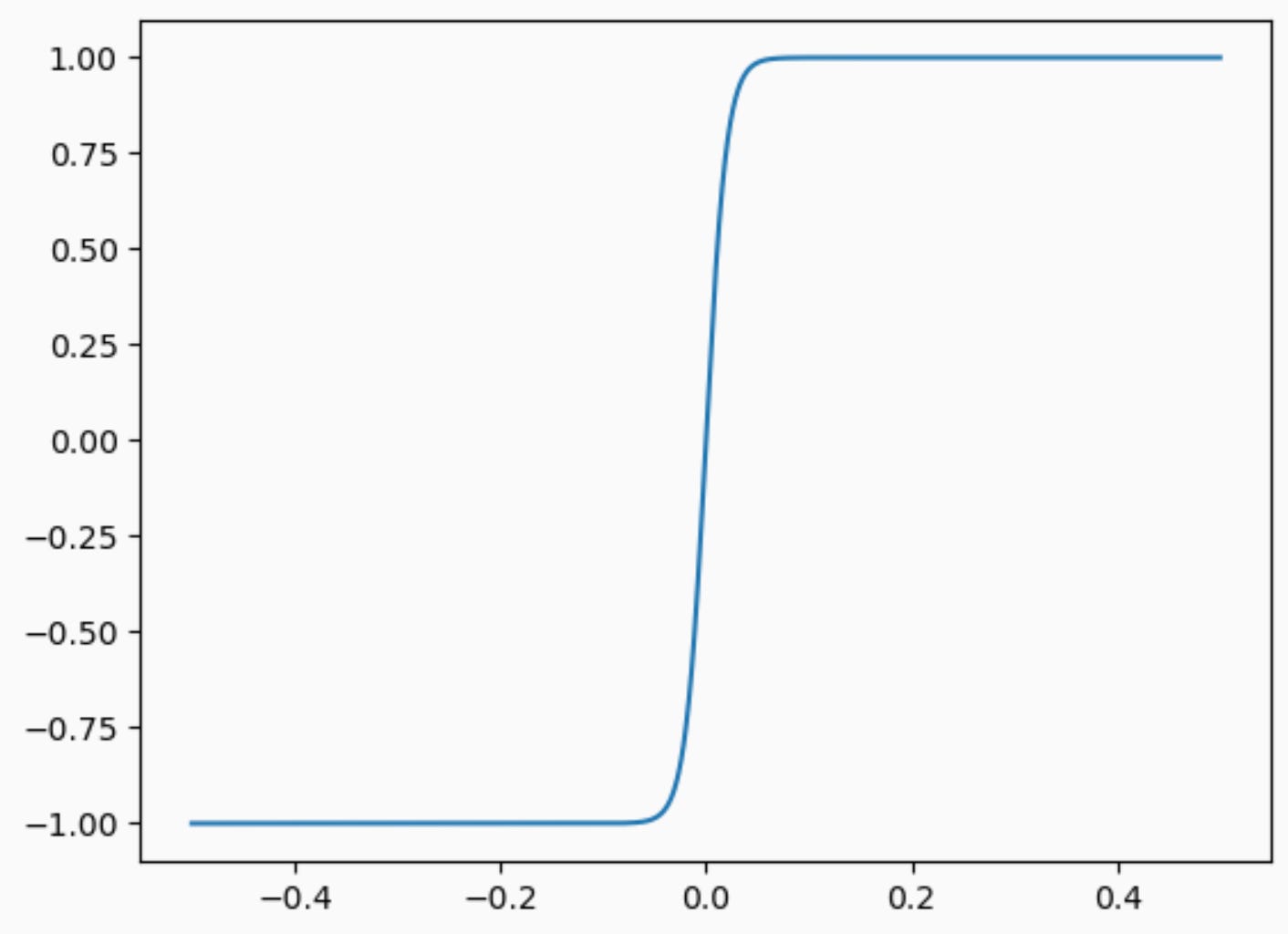
How can I characterize nonlinearities like this? All sigmoids have the property that f(x)/x is a nonincreasing function. This single, simple constraint lets us analyze the nonlinear system.

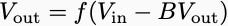
With a nonlinear amplifier, the output satisfies the equation

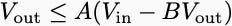
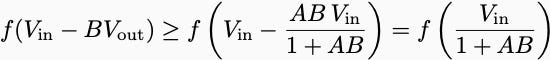
We can use our main inequality to upper-bound the right-hand side. Let A be the limit of f(x)/x as x goes to 0. Then we find

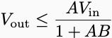
This is exactly analogous to the equation we had for the linear amplifier. Rearranging the inequality gives us the expression.

Using this last inequality, we can also get a lower bound on the magnitude of the output.

Putting this all together, we get the chain of inequalities

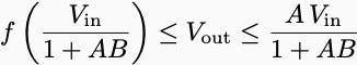
If the amplifier is high-gain, then these two nearly coincide, showing that the nonlinear feedback interconnection yields a linear amplifier with gain 1/B over a wide range of inputs. We’ve widened the set of uncertain amplifiers that we can certify in a closed loop with this one simple constraint that f(x)/x is nonincreasing. Indeed, the constraint “f(x)/x is nonincreasing” includes far more nonlinear functions than just sigmoids. As we’ll see in a couple of weeks, identifying nonlinearities with simple constraints is a powerful way to analyze feedback systems and is more or less what we’re already doing when we analyze optimization algorithms.

1. As we will see in a couple of weeks, the word almost is key here.