
Links and Loops
Feedback as the abstract algebra of interconnection.

This is a live blog of Lecture 1 of my graduate seminar “Feedback, Learning, and Adaptation.” A table of contents is here.
The word “feedback” colloquially has a dynamic connotation, where suggestions correct or steer behavior after that behavior occurs. The autonomous car senses it is moving away from a lane and sends a signal to turn the wheel to correct its heading. A human annotator slouches behind a screen rating the outputs of language models and sends the ratings back to a datacenter to improve chatbots. There is this sequential feel to feedback: action by an agent, observation by the supervisor, correction by the controller.
Control theory, by contrast, abstracts away dynamics and formalizes feedback as a particular kind of interconnection. Feedback identifies the outputs of systems with the inputs of others. This purely algebraic identification transforms all of the other signals so that the interconnected system behaves entirely differently from the original systems without the feedback. Let me today belabor the most basic problem in feedback design to demonstrate how putting two simple systems together yields unexpected, counterintuitive behavior that is surprisingly robust.1
Our goal will be to design an amplifier with a precise amount of gain using one with a large, unknown gain. All we know about the amplifier is that it makes the input larger by some amount. We might imagine that this amplification is not only unknown but potentially variable day to day. Our only commitment is a rough idea that the amplification factor is big.
With such a high-gain system, we can create controlled amplification with feedback. We take the output of the amplifier, attenuate it by a precise, constant factor, and then subtract the attenuated signal from the input signal. This creates a circuit like this:
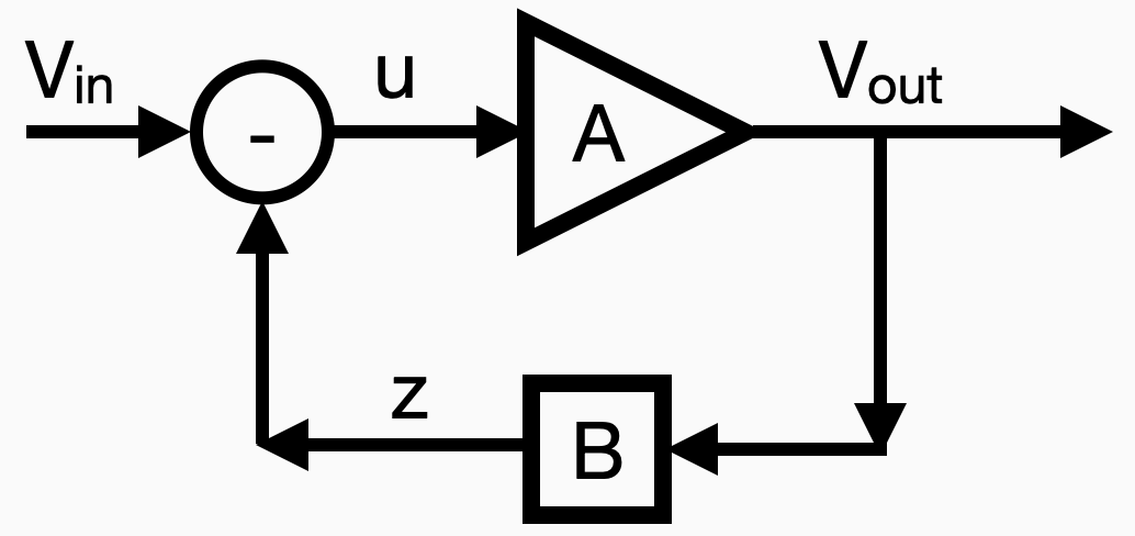
In this diagram, we have a constant reference signal, Vin, and a measured output, Vout. B is the attenuator. We connect the output of B to the input of A in negative feedback, subtracting the output of B from Vin and making this input to the amplifier. If we write all of the relationships down, we have three equations and three unknowns:

We can solve the system to find the values of u, z, and Vout. In particular, I want to focus on the relationship between the input and output:

When A is large, the gain from input to output is effectively 1/B, no matter the precise value of A. By identifying the input with the output, we get an expression that’s robust to the unknown value of A. We don’t have to precisely “learn” A to have a reasonably constant output. If B = ½ and A is any number between 400 and a million, then the closed-loop gain from input to output is, for all intents and purposes, equal to 2.
I won’t go into the gory details here, but we still obtain this robust output even after considerably generalizing the amplifier model. If the amplifier had additive noise on the output, this would be damped by feedback as long as the noise magnitude was much less than the amplification factor. A more realistic amplifier would have high gain, but would clip signals to some maximum and minimum values. First-year calculus shows that your output is approximately (1/B) times the input, provided you keep the input sufficiently small so the output doesn’t saturate the amplifier.2 This analysis is also robust to a wide range of possible saturating effects.
Though we removed all aspects of time here, this static example turns out to be a literal microcosm of the general principles of feedback. First, we can think of the signals Vin and Vout as being vectors rather than scalars and the boxes as linear maps between the inputs and outputs. All the equation solving we did today would still work out. In particular, we still get

This expression makes sense as long as the matrix I+AB is invertible, which it is as long as the open-loop map AB does not have -1 as an eigenvalue. If the eigenvalues of AB are all large and positive, this expression will also roughly be amplification by the inverse of B. Math sickos will note this same expression works even if the signals are infinitely long vectors and A and B are maps on the appropriate normed spaces, as long as that inverse isn’t singular.
Now, let’s imagine the signals are time series and A and B are convolutions. That is, assume the output is some autoregressive–moving-average model of the inputs (time-series people have assigned the fun acronym ARMAX to these models). The fun and miraculous fact is that covolutions commute (that is, AB=BA). So even if we are conceptually thinking about maps between infinitely long sequences, as long as the mappers A and B are convolutions, we can effectively treat the entire problem like a simple, static amplifier.
That’s all we do in classical linear systems theory: answer questions about dynamics with algebra. You can already see that the important thing is for the matrix I+AB to be appropriately bounded away from zero in all directions in vector space. Control theorists call this internal stability, but it just means that all of the time series remain reasonably bounded. At this point in a standard controls class, the instructor would usually break out Laplace transforms for 6 weeks and start showing you contour plots of rational functions. The reason we do this is that it makes it easy to see all the different directions in which signals might blow up, effectively reducing the problem to looking at a bunch of independent cases. What we call “frequency domain” control transforms questions about temporal dynamics into an infinite collection of amplifier problems. It’s an amazingly powerful concept, but requires unpleasant, complex analysis. I’ll spare everyone the painful details today.
Even without the more advanced math, we can see that interconnection induces an unintuitive transformation of the input-output map. Two systems that look entirely different in isolation exhibit the exact same behavior when constrained by the authority of negative feedback. Moreover, the same control policy, in this case the “attenuator,” transforms a wide range of different systems into effectively the same system. This sort of algebraic squashing through interconnection is, to me, what defines the core of feedback control theory.
For long-time readers, I wrote about this particular example two years ago on the blog.
I might add those details tomorrow. But I’m trying to minimize the mathematics in this post.
Yes and no - I saw you palm that card. By invoking the assumption that the system could be treated as linear, you assumed away the hard part of the general problem. Instead, suppose your plant is some big, complicated nonlinear causal system, and the initial condition of the system, when we first turn on the feedback loop, is nowhere close to where we want it to be - not in the linearizable close neighborhood of the desired end condition, and not even in the same basin of attraction. Let's assume for the moment that we do have good-enough causal computer model of the system, suitable for use in a model predictive control loop, but that model is not remotely close to being invertible, and there is no guarantee that there exists any possible state trajectory, under control, that will get us to the desired end condition, or anywhere very close to it, but we still want to find a way to get onto a trajectory that will get us as close as possible to it.
This is the general problem that I've been thinking about a lot lately, because it comes up in some of the most important "wicked" roblems confronting us (meaning humanity as a whole), such as how to get onto a trajectory that will carry us safely past the ongoing polycrisis/metacrisis, and into a long-term "protopian" future.
For linear systems in particular both linear algebra and geometry come together in a unified way that is unique (not possible in nonlinear systems). For the state feedback example that you showed, a geometric interpretation with the column spaces of the various matrices and how they interact could be an intuitive teaching tool for some types of students (like me).