You Play to Win the Game

The game theory behind algorithmic decision making

This is a live blog of Lecture 7 of my graduate seminar “Feedback, Learning, and Adaptation.” A table of contents is here.

The Monday after Spring Break is always a weird class with people trickling in from their various excursions. So it’s an ideal time for a weird lecture. I decided it was time for some game theory.

The goal of this seminar was to focus on the power of feedback, to understand how to think about complex interconnected systems, and to understand how feedback design allows systems to “generalize” and “behave effectively in unknown future settings”.

In classical control, you can argue that feedback is for stabilization, for maintaining fixed points, for rejecting disturbances, or for recovering from failure. We covered some of these ideas in the first part of the course.

However, there’s another view of feedback, one that’s ubiquitous in machine learning and artificial intelligence. It’s the one that’s most prevalent in the quantitative social sciences. And, increasingly, based on my interactions with Berkeley graduate students, in robotics. That is the idea of feedback as a way to augment optimization.

In optimal control, feedback is used for the most narrow-minded reason: it lowers cost. Feedback policies, because they search over a larger space of policies, have lower cost than open-loop policies. That’s it. Feedback provides more information to the decision-maker, and a decision-maker who uses information will achieve a lower cost than one who doesn’t.

The optimal control model of feedback is game theoretic with rules of engagement staged as follows:

In every round t,

1. Information x_t is revealed to both players.

2. Player one takes action u_t

3. Player two takes action d_t

4. A score r_t is assigned based on the triple (x_t,u_t,d_t).

Player One is the “decision maker,” and their action has to be computable from a few lines of code. Their goal is to accumulate as high a score as possible, summed across all rounds. Player two wants the sum of all of the r_t to be as low as possible.

Player One’s action can be computed based on the rules of the game and all of the moves they’ve seen thus far. This is why if they optimally use the revealed information, they will have no worse cost than if they throw the information out.

Player Two is “the adversary.” Their power dictates how hard the game is for the decision maker. In some formulations, Player Two chooses oblivious random actions. You can make Player One’s life harder by making Player Two an omniscient god that knows Player One’s strategy in advance and can compute undecidable functions to topple them.

If there is a single round and Player Two is random, this game is called decision theory. We’ve collectively decided that the best strategies against random adversaries are those that maximize the expected value of the score. Don’t ask me why. If there are two rounds, it’s stochastic programming. If there are an infinite number of rounds, but there is no relationship between the rounds, it’s a bandit problem. If there are infinitely many rounds and the information follows a Markov chain, this is stochastic optimal control or reinforcement learning. In this case, when the costs are quadratic, the Markovian dynamics linear, and the adversary normally distributed, this is the linear quadratic regulator problem.

When Player Two is adversarial, Player One seeks a strategy to maximize their score against the best imaginable opponent. If there is a single round and Player Two is adversarial, this is called game theory or robust optimization. If there are an infinite number of rounds, but there is no relationship between the rounds, it’s a non-stochastic bandit problem. If there are infinitely many rounds and the information follows a Markov chain, this is robust optimal control. The linear version of this robust control problem is called the H_♾️ optimal control problem. Phew!

Now, every single one of these problems requires a slightly different algorithmic solution. That’s what keeps us in business. For every gradation, the solution details can fill a textbook. But they are all variations of the same game-theoretic framework. Having been formalized in the late 1940s and honed in the military-industrial boom of the 1950s and 1960s, this game-theoretic model of control and decision-making has been standard since the 1970s.

I’m not saying any of this is wrong, per se. I am saying that it is a bit limited as a framework. Part of the motivation for this course was to make better sense of this “graph” I made in a blog series a couple of years ago.

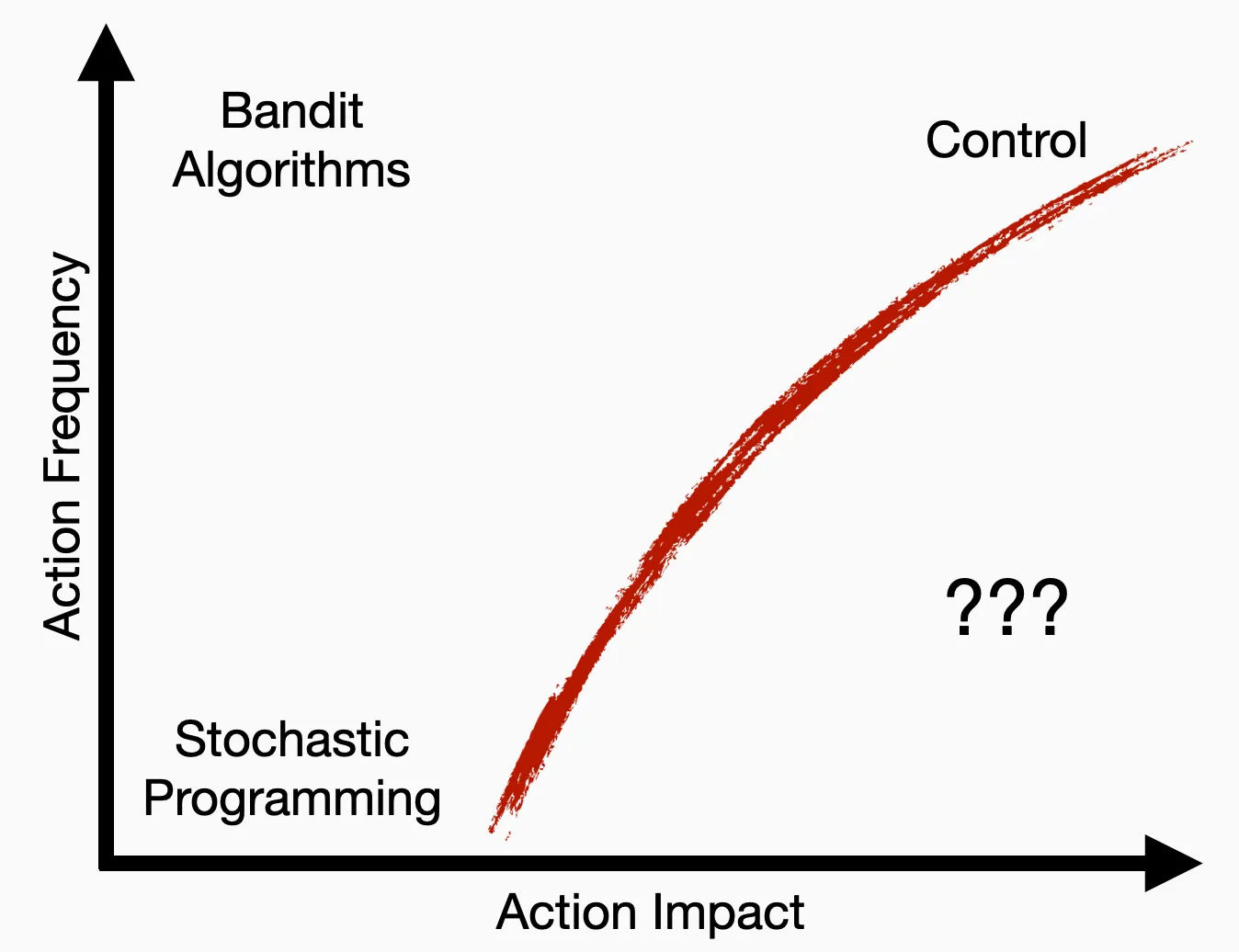
I observed that decision-making frameworks were distinguished by two variables: the impact each action had on a system external to the decision-maker (the x-axis) and the frequency with which decisions could be made (the y-axis). Game-theoretic decision making requires first figuring out where on this graph you want to operate. If you have a problem that calls for a specific level of impact and have the authority to act at a specific speed, you can find a particular solution using a proper game-theoretic formulation. How powerful you make Player Two will affect the complexity of your decision system and its conservatism. Since you have no idea what the future holds, your conception of Player Two is a subjective decision, but at least it’s one you can precisely describe. In this sense, the optimal framework is nice because you can declaratively compute decision policies based on systems modeling.

But if you have problems that span multiple regions of this space, or ones that lie below that red curve, the optimization framework gets stuck. If you have problems where the costs are ambiguous or variable, it’s hard to argue in favor of a policy based on models of cumulative reward. If you care about multiple levels of interaction impacts and speed, optimization stops being helpful.

The problem is that if you want to move into high-impact regimes where your authority is less than you’d desire, no single system gets you there. At some point, you have to think a bit more broadly about what systems push hard against this red curve. We’re forced above the red curve because of different limits, some fundamental, some conceptual. Physical law, computational efficiency, and even the ability to model keep us on one side of the curve.

I’m not sure this class helped me understand how to move beyond this curve, but it helped me understand a bit better why we’re stuck with it. The action-impact curve shows that single optimization problems can’t govern complex systems on their own. How do existing complex systems, be they natural or artificial, get around it? I’ll reserve the last two lectures of the class for this sort of abstract navel gazing.