Structured Uncertainties

A brief introduction to the structured singular value and what it teaches us about uncertainty quantification.

This is a live blog of Lecture 9 of my graduate seminar “Feedback, Learning, and Adaptation.” A table of contents is here.

The problem with a fast-paced course is that I keep hitting topics I want to dig into but am forced to move on. Simulation is fascinating, and I need to spend more time with its history and nuance. I guess that just means I’m going to add it to the syllabus of my next graduate course.¹

But I wanted to post about one fun thing I learned this week that, while not directly related to simulation, does seem to have some broader lessons. I came to better appreciate John Doyle’s structured singular value, often called by its Greek name “𝜇” or “mu.” The lessons it teaches about interconnection and uncertainty, though perhaps not always computable, are quite general and important.

Let’s go back to the recurring simple feedback loop.

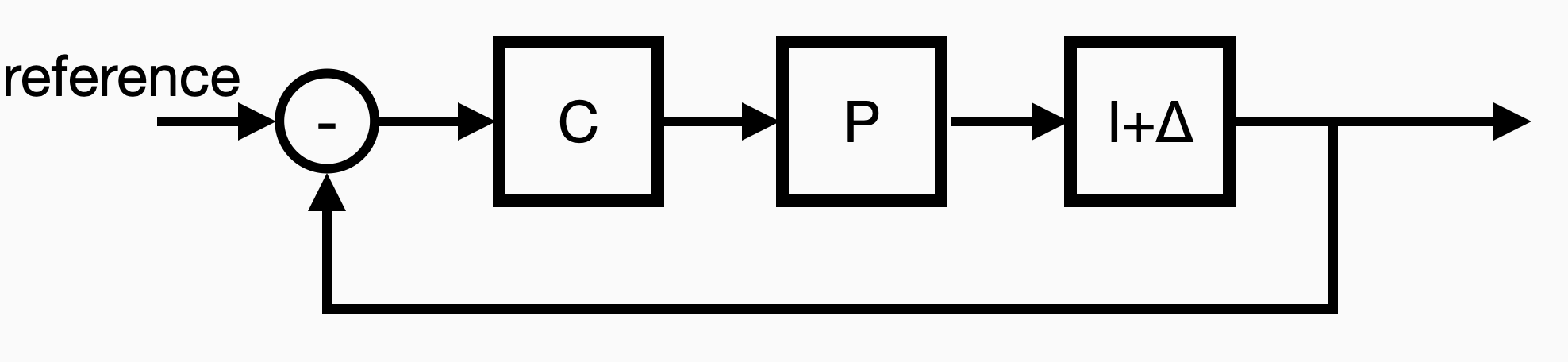
Here, C is the controller we’re designing, P is the plant we’re trying to steer. I’ve added a new block, Δ, to represent some uncertain system in our feedback loop. When Δ equals zero, we have our nominal system model. The structured singular value asks the following question: if I have a design that works without uncertainty, how much margin for error do I have? How large can Δ be before the system goes unstable?

A standard problem in linear control models Δ as a simple scalar. In that case, because of how the equations work out, the uncertainty question is about the gain margin of the linear system. How much can you amplify or attenuate the plant before the closed-loop system goes unstable? Asked another way, how well do you need to know the amplification factor to guarantee stable operation? Or, let’s say you have a bunch of plants that all have reasonably similar dynamics but different gains. Is your controller good enough for all of them? The uncertainty could model the mass of a flying vehicle or the insulin sensitivity of a person with diabetes. Steady-state control of both of these systems relies on some robustness to uncertainty.

One of the classic results about the linear quadratic regulator is that its stability is maintained for any Δ between -½ and infinity. That’s a good gain margin! Many other control design techniques from classical control using Nyquist plots can also guarantee large gain margins for single-input, single-output systems.

However, the problem becomes a lot trickier when you need to control a plant with many inputs and outputs. Most control systems are networks of interconnected feedback loops, not just simple single-input, single-output systems. In my favorite control system, the espresso machine, you might have a PID controller for water temperature and another for water pressure. You could calibrate these by tuning each PID parameter, one at a time. But obviously, these two loops interact with each other. They also interact with your grind and your tamping.

An industrial process, a chemical plant, or a robot has a networked control system of far greater complexity. You might be able to write out performance guarantees for each loop in the system, and that might look fine on its face. But if these loops are coupled, your margin calculations might be misleading.

To see why, we can look at a static example, like we did with the feedback amplifier. Imagine we’re trying to get a plant to track a constant reference signal. The controller compares the reference signal with the plant’s output and applies a new input if the difference is large. This signal sets a different set point for each loop. We can compute the steady state of our system by looking at a matrix equation. Indeed, slightly abusing notation, we can think of the steady-state maps C, P, and Δ as matrices (these are the DC responses of each system). The map from the error signal input of the controller, e, to the output of the uncertainty, y, is a system of equations:

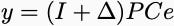
Using the fact that the error is the difference between the reference and the output, e = r - y, we can compute the steady-state output as a function of the reference signal. It’s not the prettiest formula, but you can write it out in closed form and stare at it:

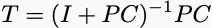
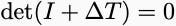
If the open-loop map from the controller input to plant output — the matrix (I+Δ) PC — is sufficiently large, the output of the plant will be approximately equal to the reference input. However, there’s a catch. We need to know that matrix never has an eigenvalue of -1 for any instantiation of the uncertainty. If it does, then the inverse in the above matrix expression isn’t defined, and the expression blows up in unpleasant ways. We’d say the closed-loop system was unstable.

Hence, we can capture a notion of multivariate robustness by finding the smallest perturbation that makes that matrix singular. The tricky part is that you get different answers based on what sorts of uncertainties you believe are plausible.

Consider the classic gain margin question. For simplicity, define the matrix

When Δ is a scalar, you are just looking for the smallest number such that

This number is precisely equal to the inverse of the magnitude of the largest eigenvalue of T. By contrast, if you think that you can have uncertainty that couples channels of your system together, the size of the uncertainty you can handle is much smaller. Indeed, you can check that if you allow for the uncertainty to be an arbitrary matrix, the norm of the uncertainty has to be smaller than the inverse of the magnitude of the largest singular value of T.

Singular values are always larger than eigenvalues. Sometimes, they can be much larger. For instance if

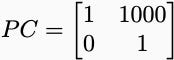
Then the eigenvalues of T are ½, and the maximum singular value of T is approximately 250. If the uncertainties were just a multiple of the identity, it would appear very robust to perturbations, handling disturbances with gains up to a magnitude of 2. However, if general matrix uncertainty were allowed, you could only handle disturbances with gains of magnitude at most 0.004.

The structured singular value lets you figure out what this magnitude is for whatever plausible model of uncertainty you can construct. Maybe only a subset of the loops is coupled. Maybe Δ has block structure. Each structure gives you a different number in between the spectral radius and the norm of your system’s complementary sensitivity, T. The structured singular value generalizes beyond this simple matrix example to general linear systems. It lets you compute bounds even when the uncertain blocks are themselves structured dynamical systems.

For people designing mission-critical linear feedback systems, you should learn all of the details. For everyone else who is stuck with nonlinear systems, there are still lessons to take away. Nonlinearity seldom makes our lives easier! If a robustness problem presents itself when we look at simple linear instances, we shouldn’t just hope that it’s not there on hard nonlinear ones. This is one of the reasons that in our post-math age of YOLO scaling, it’s useful to learn a little bit of math to be a little bit chastened. Though I suppose if you do it that way, you’ll never make a dime.

1. It is indeed already on there, my friends.