Small World Models

How much do you need to know about a system to control it?

This is a live blog of Lecture 6 of my graduate seminar “Feedback, Learning, and Adaptation.” A table of contents is here.

The backbone of control engineering is the assumption of a reasonably reliable, reasonably simple dynamical system with inputs and outputs. We have to believe that the behavior of the thing we want to steer is consistent enough so that whatever we design in the lab will work on the road.

Now, what exactly do I need to know about this reliably consistent dynamical system to get it to do what I want to do? You want a model of the system that is rich enough to describe everything you might ever see, but small enough so that you can computationally derive control policies and, perhaps, performance guarantees. Simpler system descriptions yield simpler state-estimation and control-design algorithms, both online and offline. What’s the right balance between modeling precision and simplicity? This is the question of system identification.

System identification is the natural place where machine learning and statistics meet control engineering. You need to either estimate parameters of models you believe are true or build predictions of how the system will respond to a string of inputs. What sorts of statistical infrastructure you need varies on your control engineering task

Sometimes you really believe that for all intents and purposes, the system behavior is captured by simple differential equations. An object falling in space without friction will obey Newton’s laws. To identify this system, you just need to measure the object’s mass. Easy peasy.

For more complicated mechanical systems, like quadrotors or simple, slow-moving wheeled vehicles, you still can get away with relatively simple modeling where the geometry of the problem gives you a nice differential equation with a few parameters determined by the build of your drone. In these cases, where you don’t need particularly high performance, you need only break out the ruler to scale to guestimate all of the parameters.

Sometimes you can’t determine the parameters from simple measurements, as environmental conditions dictate their values. For example, coefficients of friction might depend on temperature and the particulars of the flooring. Now you can find the parameters by repeatedly testing your system and running a nonlinear regression to minimize the input-output error.

As your problem gets even more complicated, maybe you don’t want to bother building a sophisticated simulator and would be perfectly fine with a “black-box” prediction of outputs from inputs. We’ve developed a zoo of methods to do this sort of prediction. The simplest are the “ARMAX” models, which predict outputs as a linear combination of the past inputs and outputs. You can fit these using least squares. If you want to be fancy, you can even compute nice “state-space” models from these linear ARMAX models, using a family of methods that are called subspace identification. This will yield smaller models and simplify your control synthesis problem.

On the other hand, you can go in a completely different direction and make your time-series predictor nonlinear. You can use a neural network to predict the next output from your history. If you want to get extra fancy, throw a transformer at the problem. I’m sure this will work great and build the best simulator without knowing anything about the problem at all.

So what’s the right level of modeling granularity for your problem? I don’t have a clear answer. In optimal control, the better your estimate, the better your performance. But maybe you care about the minimal amount of information you need to control something. How much is it?

You might think none. We’ve seen in class already that two systems that look completely different in open loop look the same in closed loop. Feedback can correct modeling errors. The simplest example is

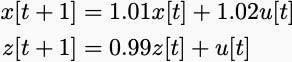
Input u[0]=1, and the “x” variable goes to infinity, but the “z” variable goes to zero. However, under the negative state feedback rule “u[t]=-x[t]”, the systems are identical

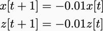
which both quickly converge to zero.

Negative feedback is powerful and can drive solid performance in the face of huge model uncertainties. If you simply care about robust tracking or homeostatic behavior, perhaps you can get away with the most minimal system identification. Unfortunately, it’s not quite that easy. You can have two systems that look the same in open loop but have completely different closed-loop behavior. Karl Astrom has a relatively simple example that I described in an earlier post. There, one system has a filter between the controller and the state that slightly attenuates the frequencies needed to stabilize the system.

Now the question is whether Astrom’s pathological counterexample—where two systems look similar in open loop simulation but are catastrophically different under feedback—is indicative of widespread problems. Probably not. I’m not convinced that you have to learn sophisticated robust control for most small-scale robotics demos. (Sorry, John, though complex aerospace systems are certainly another story). I think the takeaway from Astrom’s examples is that your model should represent the sorts of disturbances and signals you should see out in the world. And it should be cognizant of the fact that you are going to use the model in a closed-loop, so you have to understand whether there are delays and noise between the actuation signal and the actuation action.

Of course, this makes sense to any graduate student who has worked on a real robot. Every robotics grad student I’ve spoken to has told me that investing the time in system identification makes the robotic performance infinitely better. Sometimes we have to sit with our dynamical systems for a long time before we know what we need to control them. Understanding what it means for our models to be good enough is the tricky part.