The same but different

Yet another example of where good predictions still lead to bad outcomes.

In the last post, I highlighted the power of feedback in decision systems using the hundred-year-old example of the feedback amplifier. There, I showed that systems with very different behaviors looked almost identical once connected in negative feedback. Today, I want to describe the opposite phenomenon, where two systems look the same but have very different feedback behavior.

Let me also attempt to get us a bit closer to the sorts of problems people study in decision making. I’ll work today with differential equation models of decision systems. Eventually, I’ll get us back to the rigid computer science world of discrete-time systems, but let’s use some calculus today as it makes the story clean. And differential equation models are definitely commonplace in decision systems, modeling the behavior of climate, ecology, physiology, and epidemics.

Suppose I have some dynamical system I’d like to use as an amplifier. The goal for today will be to ensure it’s suitable to put inside a simple negative feedback look.  Let’s say that the true system follows the differential equations:

The input signal here is u, and the system has three internal states (x,y,z). The “dot” over the variables denotes a derivative. This system is what control theorists call stable. If you input a short signal, the output will decay rapidly. You can simulate this for yourself at home.

What would an engineer need to know to use this system as a simple amplifier? A reasonable approach would be to test the system in a controlled laboratory setting and simulate what happens when feedback is applied. They might not know that this system is a three state system, and fit a simpler, one state system to the collected data. The following differential equation, for example, will produce outputs that look very similar to the true, 3-state system:

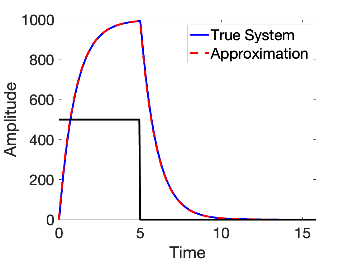
Here’s a plot of what both systems do if we apply a step input and watch the response:

They’re hard to tell apart! But what happens if we use these two systems as feedback amplifiers? To do this in differential equation land, we make closed loop differential equations by subtracting the state x from the input u. In my approximate model, the closed loop dynamics follow the differential equation. 

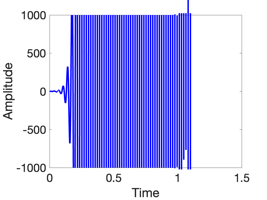
But for the same closed loop, the true system is unstable. Here’s what happens if you feed a short click into the true system when the loop is closed with negative feedback:

The system quickly blows up, amplifying a particular sine wave that rapidly saturates. This is never desired performance!

This example is getting us back closer to the theme of the current blog series. I’ve given you an example of two models that make the same predictions about a system. But when we intervene on these systems, the outcomes are very different. Could we have anticipated the bad outcome with uncertainty quantification? In order for uncertainty quantification to help, we need to understand which uncertainty can lead to undesired behavior. Can you tell me simply what uncertainty I need to quantify before I act? (I can give you an answer, but it requires Laplace transforms.)

Figuring out what exactly I need to quantify is pretty annoying. I can give you another example where two systems are completely different in open loop laboratory experiments but look identical when connected in feedback. I described similar examples in the amplifier post, but let me give you another one here as a differential equation. This is often the first differential equation you’ll learn:

This system is unstable in the open loop. If you feed in any input, the signal will blow up exponentially. But in the closed loop, subtracting x from u, we get the dynamics model

This system looks exactly like the closed loop system I described above. Two systems with completely different open loop predictions have indistinguishable closed loop behavior.

Now, what I wrote today was in terms of differential equations, but all of the examples came from this wonderful paper by Karl Astrom which presents them exclusively in the frequency domain. Every time I switch to the frequency domain, I’m sure I lose 90% of the readership. As I mentioned before, the frequency domain is a weird world of Laplace Transforms and complex numbers. But the examples in today’s post are considerably more transparent in the frequency domain. In the next post, I’m going to foolishly try to defend frequency domain analysis, explaining Astrom’s arguments.