

Hi there, argmin readers! As the fall semester picks up, posting volume will, too. So I’m going to commit to writing short descriptive headers to help you sort through the different threads. Today’s post is a live blog of Class 7 of my graduate seminar “Forecasting: A Critical Retrospective.” The syllabus and list of past posts is here.
In Kathryn Schulz’s New Yorker article, “The Really Big One,” she often cites figures about the chances of earthquakes.
“[T]he odds of the big Cascadia earthquake happening in the next fifty years are roughly one in three. The odds of the very big one are roughly one in ten.”
She described how these numbers arose by counting historical events and turning them into probabilities of the future. In the first week of class, we discussed this alchemy for clear discrete events. Coin flips, free throws, or elections have known times at which they occur. Only their outcome is uncertain. When we try to predict time, we need a new protocol: survival analysis.
Survival analysis is something I learned (and I think most people learn) in medical statistics. The name kind of gives it away: who do you think is surviving here other than patients in medical studies? In medicine, survival analysis captures the proportion of individuals still alive after a potentially life-extending treatment. Or, just as commonly, we flip this around and ask what proportion of subjects have not experienced a bad event yet.
In a randomized clinical trial, all patients start their timers at the same time—when they are randomized. The trialists gather the times from randomization until the bad events, and then estimate a probability distribution on the time until an event occurs. This distribution is over times, and is specified by a curve that models the chance the time to a bad event is greater than T. For example, this could be a distribution of how long it takes for cancer to progress under some new treatment. Or it could be how long until someone contracts an infection in a vaccine study. A survival curve lets you make probabilistic forecasts. For every time, you can look at the estimated proportion of individuals who have not yet experienced a bad event and call that the prognosis. “90% of patients experience no bad outcomes in the year following treatment.”
Here’s the most famous survival curve of all time. Who remembers this one?
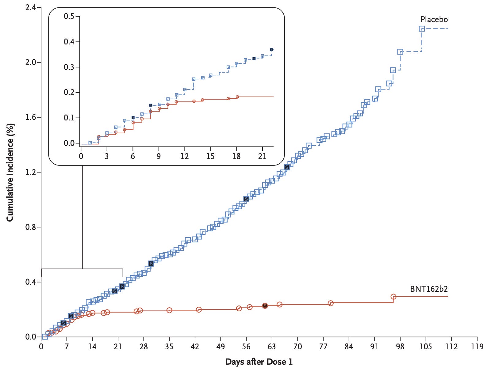
These curves are estimated using a nonparametric method called the Kaplan-Meier estimator. The Kaplan-Meier curves give a rough shape of the survival distributions and let clinicians compare the relative effectiveness of treatments. When the treatment and control curves are far apart, it suggests something meaningful differs between the treatment and control conditions.
We can apply the same survival analysis ideas to other time-to-event forecasts. Let’s caricature how we might do it for earthquakes. For a single fault, you can imagine a major earthquake as a “reset” of the tension in the earth. Each earthquake gives you a time to start counting until the next one. If we assume every earthquake follows identical geodynamics, we can treat each earthquake like a patient in a trial, now estimating a survival curve for the time to the next earthquake. This is a crude model, as it assumes a total reset of conditions, but it’s a starting point.
Once we have this model, our historical record gives us a path to estimate the survival curve and forecast the probability of an earthquake in the next T years. Although we could build a Kaplan-Meier curve here, we could also pose an explicit model of how the probability changes over time and fit the parameters.
Any probability distribution over nonnegative numbers can serve as a model for the time to event and thus be turned into a survival curve. A common distribution in earthquakes is the exponential distribution. That is, the model is that the probability that a new major earthquake happens within T years after the first one is:

The nice thing about the exponential distribution is that it only has one parameter to estimate from data, and the maximum likelihood estimate is super simple. It’s

This formula gives us a straightforward program. Look at the historical record and compute the average waiting time between events, W. If you want probability forecasts over time windows, treat this average time as the inverse of the parameter of the exponential distribution. In this model, the probability that there will be a new event in T years is

This model is too simplistic, but it’s the first back-of-the-envelope calculation people do, and it’s where all the figures in Schulz’s New Yorker article come from.
This exponential survival model is the same as modeling earthquakes as a Poisson process. You can get fancy and make your model more sophisticated to capture more physical reality, specializing parameters to the particulars of each fault. You can model the survival function with some other distribution, be it log-normal, Weibull, or whatever. However, every modeling assumption you make adds more parameters to fit from data, and earthquakes don’t occur frequently enough to fit that many parameters to reasonable precision. If you have only forty events, you should probably estimate only one parameter.
Whatever modeling you do, survival analysis gives us another apparatus for turning counts into chances. How precise you think those chances are now rests on a whole lot of untestable modeling assumptions. What is the chance those assumptions are wrong?
"What is the chance those assumptions are wrong?" Oof. What a difficult question despite its simple statement. A frequentist frames this as: count the cases in which those assumptions are wrong and divide by the number of cases in which those assumptions are wrong plus the number of cases in which they're right. A Bayesian says: state the number between 0 and 1 that you believe in. Neither offers a number indicating "I don't know." I personally lean toward a qualitative assessment in practice that asks: why might those assumptions be right or wrong? And if we're lucky, the answer to that question leads to an experiment that we agree might provide evidence one way or the other. Otherwise, I'm paralyzed and muted by Humean skepticism.
The forty-events example makes the trade-off very concrete. It’s easy to read a precise probability and forget how much of that precision came from the chosen model, rather than the observations.