Universal Cascades

A little approximation theory goes a long way

This is a live blog of Lecture 9 of the 2025 edition of my graduate machine learning class “Patterns, Predictions, and Actions.” A Table of Contents is here.

In the last class, I tried to describe this general shape of contemporary machine learning maps. To make predictions, we assemble data into boxes of numbers, and then iterate between a form of “template matching” and “column pooling.” Don’t take these two scare-quoted operations literally, but you can think of what a transformer does as something like this alteration. This gives us a reasonably simple design pattern. I then wrote, “The only theory about data representation that I’m comfortable with, I’ll discuss in the next lecture: how to efficiently generate nonlinearity maps on vector spaces.”

I’m not sure I’m that comfortable with this, but I can certainly say generating nonlinearity is easy. What do I mean by nonlinear? The problem is that nonlinear is only defined by negation. If I want a linear function in d variables, I know exactly what it looks like:

A linear function is just going to be a weighted sum of your variables. But what a bout a non-linear function? It can be anything that doesn’t have this form. That feels too general. Weirdly, the simplest little tweak on the above expansion effectively gives you all nonlinear functions.¹ If you allow yourself linear maps and only a single nonlinear function that maps scalars to other scalars, you can approximate almost anything.

For simplicity, I’ll focus on single-variable functions today. Doing this sort of analysis in higher dimensions is perhaps too complicated for an argmin post, but it’s not too bad. In this univariate case, I claim you can approximate any function with an expression that looks only a bit more complicated than the linear function I just wrote down:

x is one-dimensional in this expression. In the linear case, f would only have two parameters. In the nonlinear case, you have 3B+1 parameters to mess with. You should even think of B itself as a parameter. The function “a” is called an “activation” in neural net land. I loathe that we let neuroscientific metaphor pollute our jargon, but I can’t deny that the neuroscience artificial intelligence camp has undefeated branding skills.

No matter, let’s get to the interesting point: It turns out that almost any activation function lets us approximate almost anything. This result is both a profound statement about how simple universal computation can be and a trivial statement in functional analysis that you might learn in AP calculus.

Now, not all nonlinear activation functions give rise to universal approximation methods. If a(t)=t², the expression above will always be a quadratic function of x. If a(t)=t⁴, it will always be a quartic function. You need something other than polynomials. Though polynomials are what everyone learns in freshman year of high school, it turns out that you only need to move to sophomore trigonometry to get universal approximation.

Let’s think about what happens when a(t) = cos(t). In this case, I can pick very particular values for the weights. I can let

and now I have a Fourier series. We know that a Fourier series can approximate any continuous function on the unit interval if we have a long enough expansion. We don’t even need to search for the values of the hidden weights. We have a nice formula that will give us the values of the c_k, which we can compute by churning through some integrals.

Next, assume that the activation is a “bump” function that looks like this:

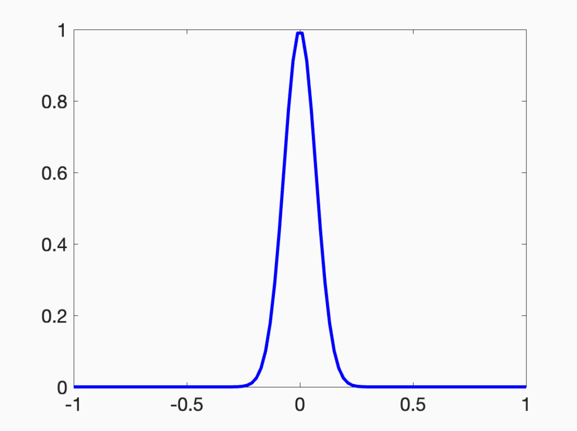
I don’t really care what the functional form of this bump is. You could use

if you’d like. You can hopefully imagine how to approximate any function with a combination of such bumps. You can dilate the bumps to make them as local as you’d want, place the bumps on the real line at appropriate points, and then multiply the bumps to approximate the values of your target function.

Finally, let’s assume a(t)=max(t,0). Now we have a “neural network with a rectified linear unit activation.” This is a bit more peculiar, but note that if we write

This function is a “bump” centered at the point v.

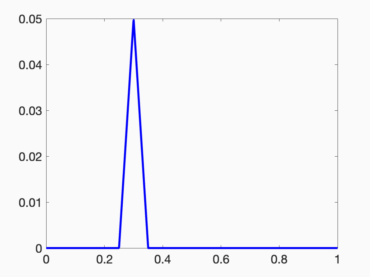
By scaling and translating this bump around, I can again approximate anything.

In fact, it’s a theorem that as long as you can approximate bump functions, you can approximate anything. Fixed degree polynomials don’t give you universal approximation, but almost anything else does.

The big question is how many terms do you need in your expansion. If functions wildly vary from point to point, you need a lot of Fourier coefficients to get a good approximation. Unfortunately, no matter what people tell you, no one knows what the functions people approximate with modern neural networks look like. Theorists have toy models in papers where they show that one architecture outperforms another. But if they had a truly dispositive model of what real data looks like, they would just fit the parameters of the model. If you have Newton’s Laws, you’re going to use them.

So we’re a bit stuck when trying to build a prescriptive theory of function approximation. We know that we can make any nonlinear function with a simple univariate nonlinear function and linear operations. To be fair, we can compute any Boolean function with linear fan-out and NAND gates. Nonlinearity cascades rapidly. In machine learning, we rest on the fact that we can build general templates for signal processing with linear cascades and selective nonlinearity. We now have a general architectural pattern. We’ll see next time that we also have general-purpose search methods for fitting these cascades to data.

1. For the math pedants out there, just relax and say “dense in the continuous functions.” It’s important not to get too shackled by mathematical rigor in machine learning.