
Stuck in the middle
Unavoidable tradeoffs in detection theory

This is a live blog of Lecture 5 of the 2025 edition of my graduate machine learning class “Patterns, Predictions, and Actions.” A Table of Contents is here.
We had a lively and enlightening discussion in class on Tuesday about how to assign costs in decision theory problems. To find an optimal decision rule, you have to precisely specify the costs associated with mistakes. These mistakes could be false positives, where you predict 1 but the actual outcome is 0, or false negatives, where you predict 0 but the actual outcome is 1. Sometimes this is easy. Maybe you just want to minimize the number of mistakes, so you equally penalize false positives and false negatives. Perhaps you are gambling,1 in which case you have literal monetary values assigned to each type of mistake.
Most problems don’t have this convenient mathematical form. One of the students asked me to write down the costs for cancer detection. What a great question that is! Suppose you have a healthy patient in a hospital system who comes in for their annual checkup. You are thinking about offering them one of these fancy new full-body cancer screens. Your thinking is that there is a large cost associated with not knowing that a healthy person has cancer. If you don’t find the cancer early enough, they might need expensive, painful treatments and might die. So what is the cost associated with the cancer screen failing to detect cancer? What numerical value would you assign?
You might say it doesn’t matter; missing cancer is so costly that we don’t need to have a precise cost associated with a missed detection. However, false positives are not costless. Taking a healthy person and labeling them with a false cancer diagnosis results in unnecessary treatments that are taxing and toxic. These treatments also have literal (exorbitant) monetary costs. Moreover, false diagnosis adds immeasurable stress to the life of the person and their family.
The costs in the cancer detection problem are at best imprecise and at worst not quantifiable. Add this to the problem of where we probably don’t have accurate estimates of cancer incidences either, and now we’re stuck in a world of “we’ll just pick some threshold on our test and that will set the guideline for a follow-up.”
And of course, that’s the world we’re in. We saw in the last lecture that testing when you have a precise cost function for average loss, the minimizing rule is a likelihood ratio test or a posterior ratio test (I’ll just call it a probability ratio test from here on). The ratio was thresholded by a number defined by the costs and prior beliefs about positive and negative rates. If we’d prefer not to specify these costs and priors, we can explore what probability ratio tests do when we tune the threshold parameter and hope for the best.
This puts us in the world of “Neyman Pearson Testing.” In the hypothetical population on which it will be applied, every probability ratio test has an associated number of false positives and true positives. There are two kinds of errors we care about. The false positive rate (FPR) is the fraction of the time a test predicts a positive outcome when it’s actually negative. The false negative rate (FNR) is the fraction of the time a test predicts a negative outcome when it’s actually positive. By century-old convention, we don’t usually talk about the FNR, but rather its complement, the TPR. The true positive rate (TPR) is the proportion of times the test predicts a positive outcome when the actual outcome is positive. The TPR is equal to 1 minus the FNR.2
The best you could hope for with these two error metrics is to have a TPR of 1 and an FPR of 0. In that case, your predictions are always correct. Whenever the outcome is positive, you are predicting a positive, and when the outcome is negative, you are never predicting a positive.
Unfortunately, perfectly clairvoyant predictors are hard to come by. The TPR and FPR are competing objectives. If you always predict “positive,” then your TPR is 1, but your FPR is also 1. Similarly, if you always predict “negative,” then your TPR is 0, and your FPR is 0. If you just flip a biased coin, which is heads with probability p, and predict positive, then the TPR and FPR are both equal to p. We thus have a baseline for pairs of TPR and FPR.
For a probability ratio test, every value of the threshold has a TPR and an FPR. Hence, we can trace out a curve varying the threshold from 0 to infinity. This curve looks like this:
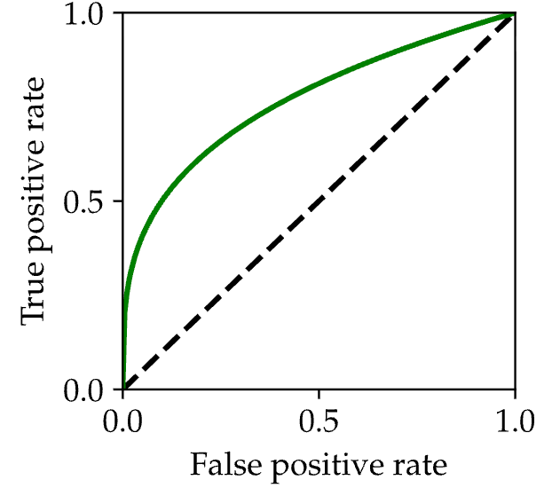
When the threshold is 0, the predictor always predicts a positive. When the threshold is infinity, the predictor always returns negative. In between, there is a concave curve, lying above the curve from the “random coin flip test” I described above. A really good probability test will have more area under it.
The curve above is called a receiver operating characteristic. Radar engineers of the Cold War invented this plot as a diagnostic for their detection systems, which were looking for signs of impending nuclear attack. As you can only imagine, it was hard to put a numerical value on false positives and negatives. This curve served as a substitute for precision cost-benefit analyses. It illustrates that for a fixed value of the false negative rate, there is a best achievable true positive rate.
Receiver operating characteristics are now abbreviated as ROC curves.3 ROC curves illustrate the first trade-off in this course. Unless your classification algorithm is perfectly discriminating, there is always a tradeoff between true positive and false positive rates. How you pick that tradeoff is a tricky balance that depends on the particulars of your problem. But the fact that the tradeoff exists is the critical takeaway. Whenever you optimize one metric, you are necessarily neglecting some other metric. How you balance the tradeoff can’t be determined by math.
The argmin blog strongly advises you not to gamble. Delete the apps, my friends.
An exercise left to the reader.
In papers, people like to brag about the area under their ROC curves (AUCROC, and I’ll stop with the acronyms for today). While AUCROC tells us something about the discriminating capability of a pair of likelihood functions, it’s one of the more blindly abused metrics in machine learning. It’s yet another convention that we’re stuck with, even though it’s not a good scoring rule.
Nostalgia: We (older generation EE folks) have learned this topic from Van Trees' textbook. His wiki page says that "Van Trees was initially on loan to the government by MIT; he then ended up staying for a number of projects." https://en.wikipedia.org/wiki/Harry_L._Van_Trees . Shame on MIT loaning a professor for money, which year is that? I think that explains why he had published rarely after his famous volumes on the topic. I have some friends utilizing his chap. 2 of vol.1 for their entire professional career (Vol. 1: https://www.amazon.com/Detection-Estimation-Modulation-Theory-Part/dp/0471095176/ )
Really like this topic because it makes a lot of engineering students uncomfortable.
"How you balance the tradeoff can’t be determined by math." That’s the most interesting part of building models, because it comes down to how they’ll actually be used. Take cancer detection: it’s rare that an AI tool is the sole arbiter of a diagnosis. Clinicians use it to guide follow-up steps.
What they really care about is, "In deployment, when the model says someone has cancer, do they actually have cancer?" That’s the positive predictive value. If PPV is low, they get alert fatigue fast and stop paying attention. And PPV isn’t just about the model, it also depends on prevalence. For rare conditions, even a model with good TPR and FPR can have such a low PPV that nine out of ten alerts are false.