

Hi there, argmin readers! As the fall semester picks up, posting volume will, too. So I’m going to commit to writing short descriptive headers to help you sort through the different threads. Today’s post is a live blog of Class 4 of my graduate seminar “Forecasting: A Critical Retrospective.” A table of contents is here.
Our first modern case study is weather forecasting. This is one of forecasting’s greatest success stories, and it’s worth pulling apart how it came to be. Max Raginsky pointed me to a fun passage in Game-Theoretic Foundations for Probability and Finance by Shafer and Vovk, noting that in the 19th century weather forecasters were called “weather prophets,” and only in the 20th century did they change their name to claim an air of scientific authority. Forecast sounds more authoritative than prophecy or prediction.
Indeed, the main turn in weather forecasting in the 20th century was toward physics. American Cleveland Abbe and Norwegian Vilhelm Bjerknes proposed using the laws of physics to forecast the weather, just like astronomers do to forecast the future positions of planets. After all, at its core, the atmosphere was just a giant ensemble of gas and fluid. If we could measure the initial state of all of the particles, we could run Newton’s Laws forward in time and exactly predict the weather for the rest of time.
Now, though they were strong believers in determinism, Abbe and Bjerknes were not that naive. They knew that they’d need to lean on thermodynamics and fluid dynamics. And they knew that even at these higher levels of abstraction, solving the differential equations by hand was out of the question. But they proposed a reasonable program: (a) measure the current state of the atmosphere to as high a precision as possible, (b) use whatever computational means possible to run a physics model forward in time. This is what we still do today.
Obviously, computation is key. From the beginning of modern computing, weather forecasting has been one of the driving frontier applications. It is an ideal application for hyperscaling because computers are never big enough to give us the global precision needed to predict whether I’ll need an umbrella two weeks from now. Weather forecasting was one of von Neumann’s favorite application problems for computers, and some of the earliest modern forecasts were demonstrated on the ENIAC in 1950. With each generation of new computers, our forecast horizon improves, to the point where 3-day forecasts are now remarkably prophetic.
Here’s a chart of the current skill of high-resolution weather forecasting. The y-axis is the “Anomaly Correlation Coefficient”, which measures the correlation between a forecast atmospheric condition and the measured deviation from the seasonal average. From 1985 to 2020, we gained about one day of forecast accuracy every 10 years. This is a remarkable success story of computational scale. In 100 years, with multiple doublings of computer power, we turned a curious scientific pipe dream into a global predictive infrastructure.
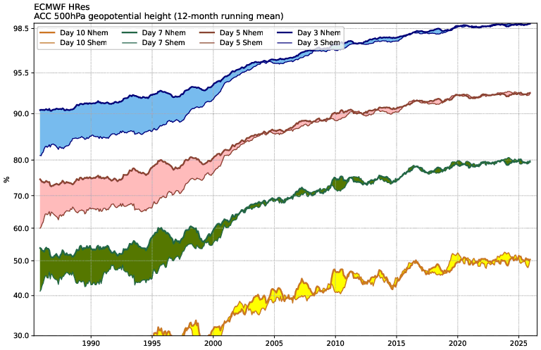
However, those gains look like they’re plateauing. Part of what makes weather forecasting so interesting is that we can predict out a few days with striking accuracy using global-scale measurement infrastructure and supercomputers. But it might only be predictable to a certain point.
Lorenz famously demonstrated that simplified weather models were chaotic, meaning two nearby trajectories diverge exponentially quickly over time. Weather models empirically display a similar property, and any small initial measurement uncertainty means that there will eventually be huge forecast uncertainty. The exact time scale of what is predictable isn’t clear, but progress on 10-day forecasts does look a bit stuck in the graph above.
One thing I find fascinating is how this uncertainty from a deterministic equation becomes probabilistic. Chaos is not randomness. Completely deterministic equations exhibit the “diverging trajectories” phenomenon. You can run fun simulations with the logistic map:
x[n+1] = 3.9 * x[n] * (1-x[n])The output sequence will look like random noise, and two close initial conditions quickly end up in completely different places after a few steps. No random number generators are required.
So where does the “chance of rain” come from? It’s a multi-step process. Probability enters because, despite global investment in measurement, we can’t perfectly nail down an initial condition to start our weather simulation. Measurement quality is better where population density is higher, as populated areas are where it’s easiest to put weather stations. However, you need high resolution everywhere to have a perfect model, and there’s still very uneven coverage. And the measurements themselves of course have inaccuracies. Backing out the state of the atmosphere from the measurements we have is not an exact formula.
So weather forecasters use estimation algorithms, including Kalman filtering techniques, to compute probability distributions of the current state of the weather from the best available measurements. I haven’t found a good discussion of why these probabilistic methods are preferred or how we should interpret the associated probabilities, but this is where probabilities enter the forecast: they use probabilistic tools to translate measurement and modeling uncertainty into a generative probability distribution of initial conditions. They can sample from this distribution and run several simulations simultaneously, thus producing a few dozen candidate “samples” of what the future will look like.
With these samples, forecasters can then count frequencies of events in the sample. If it rains in 40 out of 50 samples, they say “the chance of rain is 80%.” Is this a valid probability? Not really, because the modeling assumptions introduce all sorts of biases. So weather agencies adjust probabilities based on past events so forecasts are calibrated.
We’ll talk more about calibration on Thursday. For forecasters, they’d like you to interpret this roughly as “in all of the historical records when the atmospheric conditions were like this, precipitation was observed 80% of the time.” A forecast is calibrated if the rates in the historical forecast match the rates in the historical observations. A calibrated forecast means that it rained on 80% of the days when the forecast chance of rain was 80%. Similarly, it only rained on 20% of the days when the forecast chance of rain was 20%. Calibration is much weaker than the forecast skill plotted above. If it rains on days starting with T and you always predict a 28.6% chance of rain, your forecast is calibrated but missing the forest for the trees. Still, calibration is a nice thing to have in a weather forecast because it pins down what the forecaster means by chance of rain. Whether this interpretation of probability has any profound effect on your life is uncertain.
> I haven’t found a good discussion of why these probabilistic methods are preferred or how we should interpret the associated probabilities
The reason is a bit subtle yet interesting: it's a practical trade-off and cleanliness of interpretation is not the primary goal! From what I understood from NWP folks, in ensemble forecasting the basic goal is not necessarily to be "distributionally accurate", although it can work in that sense as a quite rough first-order rule of thumb. Since each individual simulation ("member") is computationally expensive, you want to see as many diverse plausible scenarios as possible from that limited budget, rather than spend most of your CPU cycles just simulating minor deviations from a central scenario. Hence they use techniques like breeding / singular vectors (or, contemporarily, variational assimilation) to stimulate the fastest-growing perturbations and try to catch the main modes of the variability. They are more like "probes" of the dynamics of the system than a method that explicitly targets a rigorous probabilistic distribution of the system, so there is no natural probabilistic interpretation of raw ensemble output. Hence, as you say, the need for post-processing and calibration in most applications.
Cool CA, AKA Hotter Than The Hinges To The Doors Of Hell, is the coolest town in California.