Arbitrary Geometry

Adversarial regret as a proof technique in learning, optimization, and games

This is the third live blog of Lecture 7 of my graduate seminar “Feedback, Learning, and Adaptation.” A table of contents is here.

I closed yesterday’s blog with a cliffhanger, promising to give a few examples of where I think adversarial regret is a useful concept. On its own, I’m not sure that it is a useful concept. More on that next week! But today, I’ll show how you can use adversarial regret to bootstrap interesting arguments linking machine learning, game theory, and stochastic optimization.

Once again, I list the rules of the game. We have a two-player game with repeated interactions. In every round t,

1. Information x_t is revealed to both players.

2. Player One takes action u_t

3. Player Two takes action d_t

4. A score r_t is assigned based on the triple (x_t,u_t,d_t).

Player One is the “decision maker,” and their action has to be computable from a few lines of code. Their goal is to accumulate as high a score as possible, summed across all rounds. Player two wants the sum of all of the r_t to be as low as possible.

The adversarial regret compares the score of Player One’s strategy to that of a player who sees the entire sequence of disturbances but must play the same action at every time step. It’s a weird setup where we are comparing a player who can change their strategy arbitrarily to an omniscient player forced to play the same move every time. While these two notions don’t seem worth comparing at first blush, there are a few cases in learning theory and game theory where the comparison is mathematically powerful. It turns out that computing these regret bounds is often quite simple, and they follow from elementary derivations. While these bounds themselves might not be useful, they then imply results you actually care about. Let me give my three favorite examples.

Online learning and PAC Learning

Online learning is the case argmin readers will have already encountered if they followed my machine learning course blogging. I like to teach online learning because adversarial regret bounds imply the standard model of probabilistic machine learning. Adversarial regret highlights how most of the “generalization bounds” we derive in machine learning are artifacts of geometry rather than mystical manifestations of mechanical epiphany.

In the online learning model, the goal is to predict the disturbance from the information. The actions are predictions. At each round, your score is high if your prediction is correct and low if the prediction is incorrect.

Let’s change the notation to match the standard verbiage of machine learning. The prediction is a function f, and the “disturbance” is a “label,” denoted y. Instead of a high score, we want low loss. In the online learning setting, you get to change your prediction function at every time step and compare your losses to a single model that tries to fit the labels after you see them. In equations, this is

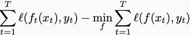
You can now do math and show that this expression is bounded by a sublinear function of the number of rounds. This post works out the details. Now, the resulting deterministic bound is necessarily interesting in and of itself, but the magic happens when you declare the xs and ys to be generated by a stochastic process. If, for example, you assume the information-label pairs are identically distributed, independently samples from some data-generating process, then after making a few assumptions about convexity, the regret bound becomes a generalization bound:

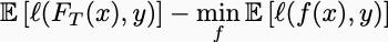
Here, F_T denotes the random function that your model returns after seeing T examples. This bound compares the predictive accuracy of your algorithm on a new sample to that of the best function computable given the data-generating distribution. If you have sublinear regret, then this quantity tends to zero as T goes to infinity. This is called a generalization bound, or, if you use probability instead of expected values, a PAC Learning bound.

The technique of deriving a deterministic regret bound and transforming it into a probabilistic generalization bound by taking expected values is called “online-to-batch conversion.” It is one of the favorite tricks of learning theorists.

Stochastic Optimization

Similar techniques can be applied more generally to stochastic optimization. A clever analysis of the stochastic gradient method takes a similar approach: you can prove that gradient descent has low regret even if Player Two is handing you a different convex function at every time step. If you take expectations of the resulting regret bound and apply Jensen’s inequality, you derive a bound on the sample average approximation method for stochastic programming. Though substantially more general, the proof is almost identical to the one in online learning.

Repeated Games

Still closely related to but slightly more challenging than online convex optimization are repeated zero-sum games. In this setup, each round of the game is itself a zero-sum game. The players battle each other for multiple rounds, and Player One’s goal is to refine their strategy so they eventually achieve an infinite ELO score. Here, a classic result proves that when both players use algorithms with low adversarial regret, they converge to a Nash equilibrium. You assume that both Player One and Player Two are using algorithms that yield low regret against an arbitrary adversary. The baseline is a player forced to use the same strategy every round. If Player One and Two’s strategic improvements have sublinear regret, their strategies eventually converge to an equilibrium. This result is the backbone of modern poker bots, which use algorithms like counterfactual regret minimization. Whether or not you think solving poker is a major contribution to humanity and human knowledge is up to you.