The maddening nonlinear multiverse

The paths to nonlinear prediction all lead to the same place

Last week, we discussed various ways to fuse measurements into descriptive features for prediction. With these features, we could fit a linear predictor and hope it gives good results on the test set. But what if we still don’t get the test error low enough to win the Kaggle competition? What do we do?

I have several answers! We could collect more data and see if we can get a more representative sample of the decision space. We could think about the prediction problem’s intricacies and design new measurements that would be more informative about the prediction task. But those both seem too hard. Is there anything else we can do just by writing more code? 

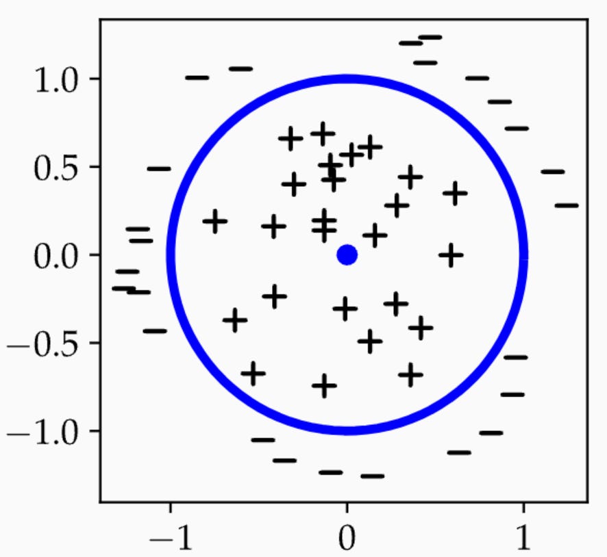
It seems reasonable that we could capture more patterns by allowing for nonlinear rules. The classic motivating story for nonlinear prediction is the following cartoon (borrowed here from Chapter 4 of PPA):

I can’t separate the pluses from the minuses with a linear function. But I can separate them with a quadratic function:

\(x_1^2 +x_2^2 -1\)

This function is nonlinear in the features and perfectly separates the data.

Is real data like this cartoon? It’s unclear. You can rarely stare at your data and see obvious nonlinear separations like this. So machine learning researchers have developed hundreds of ways to make nonlinear rules, hoping one of them will regularly win out. With hindsight, however, these schemes are all doing the same thing. You create more features using some simple, nonlinear rules. Then, you find the best linear predictor with your new feature set. Let me expand on this with a few popular ways we build up nonlinear predictors.

Taylor’s theorem tells us that every differentiable function can be approximated as a sum of polynomials. As I foreshadowed, a polynomial is a sum of monomials, and each monomial is just a product of features. Monomials are themselves descriptive features of data. If you multiply two binary features, this is their logical AND. Monomials are descriptive combinations of features, polynomials are linear combinations of them.

We could take any generic logical expression about a feature list and call this a feature. For instance, a new feature could be the truth value of a series of if-else statements. Such features are called decision trees. We could build nonlinear predictors out of sums of decision trees. This is what XGBoost does.

Since we’re just looking for sums of simple nonlinear expressions, we can think more generally about basis functions for nonlinear prediction. Again, there are many possibilities.

Radial basis functions put little bumps around particular points in space and then approximate functions by summing up these bumps. Here’s a cute picture again from PPA showing how you can approximate a sinusoid with bumps around some anchor points:

In one dimension, a bump function equals the difference between two sigmoidal functions. So I could have sigmoids along random dimensions and approximate all sorts of functions that way too. These are old-school neural nets.

Fourier analysis says that many functions can be approximated as a sum of trigonometric functions

\(f(x) \approx \sum_{i=1}^B w_i cos(\langle a_i, x \rangle + b_i)\)

This expression implies a compact form for high dimensional basis functions. A basis function can be a nonlinear function of a dot product with some vector. This, again, looks a lot like neural nets.

No matter whether we use trees or radial basis functions or splines or wavelets or neural nets, we find ourselves building nonlinear functions as sums of basis functions. We can think of nonlinear prediction as nonlinearly mapping features into a higher dimensional space where our data may be more robustly separable.

But how many dimensions do we need? Since we care about computational efficiency, we don’t want to choose too many basis functions. We want just enough to get the test error small. There are several approaches to finding parsimonious representations, and there’s no “right” answer. They all complement each other. Other constraints about hardware, software, downstream deployment, or religious beliefs will usually be why you’ll choose one over the others.

Kernel methods squash all of the basis functions down into a set equal to the number of data points:

\(b’_i(x) = \sum_{j=1}^B b_j(x) b_j(x_i)\)

This gives a reduced basis set that can still fit any nonlinear function to the training data. If I have n basis functions, I should be able to fit any pattern I’d like. Moreover, the sum here often has a clean and compact expression.

\(k(x,z) = \sum_{j=1}^B b_j(x) b_j(z)\)

Is called a kernel function. I could write a whole blog about kernels, and maybe I will…

But before that, let’s look into other alternative ways to get compact basis expansions. An alternative to kernel methods is to just pick a random collection of the basis functions. It’s unintuitive, but if all we care about is the sum of products, it seems reasonable that a random sample from this sum will approximate the sum. If I choose m basis functions at random, then the law of large numbers suggests that

\(\frac{1}{m} \sum_{i~\text{random}} b_i(x) b_i(z) \approx \frac{1}{B} \sum_{j=1}^B b_j(x) b_j(x_i)\)

This is the main idea behind random features.

A third approach would be to choose basis functions sequentially, trying to improve our predictor one basis at a time. We could keep adding promising basis functions if we’re not happy with the current prediction quality. This is what we do in boosting.

And finally, you could probably get the most parsimonious description if you searched for the best bases. At this point, we’re back to neural nets again. The only question is whether we can perform this search efficiently and effectively, as the search problem looks hard. We’ll dive into this on Thursday.