Searching for Stability

The theoretical and pedagogical links between optimization and control

This is a live blog of Lecture 3 of my graduate seminar “Feedback, Learning, and Adaptation.” A table of contents is here.

I could teach an entire semester-long graduate class on gradient descent. First, I’d present gradient descent. Then I’d move to accelerated gradient descent. Then I could teach stochastic gradient descent, coordinate descent, projected gradient descent, proximal gradient descent… This would get us to Spring break. We could wrap up the semester with other assorted gradient potpourri. Indeed, Steve Wright and I packaged this course into a textbook: Optimization for Data Analysis.

Steve and I were inspired by the thousands of machine learning and optimization papers of the 2010s that made minor extensions in this gradient zoo. All of these papers proved their methods worked in the same way. They set up a Lyapunov function. They showed that it decreased as the algorithm evolved. QED.

Those Lyapunov functions were sometimes easy to come by. You’d always start with the function value itself. If it significantly decreased every iteration, then the algorithm would converge. You could also study the distance of the current iterate to the optimal solution. It took me a decade of beating my head against Nesterov’s inscrutable estimate sequences to realize that he was actually using a Lyapunov function too. In Nesterov’s accelerated method, this Lyapunov function has the form:

Showing functions like this were Lyapunov functions required pages of calculations, but all of these were manipulating exactly two inequalities. The most important assumption when analyzing gradient descent is that the gradients are Lipschitz. This means that the slope of the gradient function is bounded. Oftentimes, we also assume that the functions are strongly convex. This is equivalent to assuming the slope of the gradient function is bounded below.

Together, we had that the following two inequalities were true for any x and z.

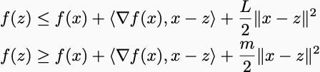
Here, L is the Lipschitz constant of the gradient. m is the strong convexity parameter. Sometimes we’d use the second inequality with m=0. You might call those functions weakly convex. Convergence proofs cleverly sum up these two inequalities evaluated at different points in space to show that some Lyapunov function decreases. After enough Tetris-like puzzling, you surely prove that the Lyapunov function decreases.

These analyses appear to be assessing the stability of a dynamical system. That’s because they are. Gradient methods control a nonlinear system that takes a vector as input and outputs the gradient of a convex function evaluated at that vector.

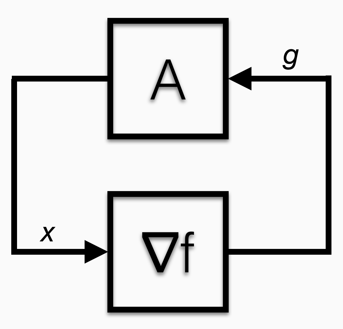
The algorithm feeds “x” into the black box. The black box spits out “g.” The algorithm does some thinking and spits out another x. Eventually, the g emitted by the black box is always equal to zero.

In fact, all of the gradient-based algorithms are equivalent to PID controllers. Gradient descent is literally an integral controller. It is even after the same goals: gradient descent wants to find a point where the derivative is zero. Integral control seeks zero steady-state error. Accelerated methods are PID controllers. Projected gradient is a PI controller.

What if we just relabel that picture to align with control theory notation:

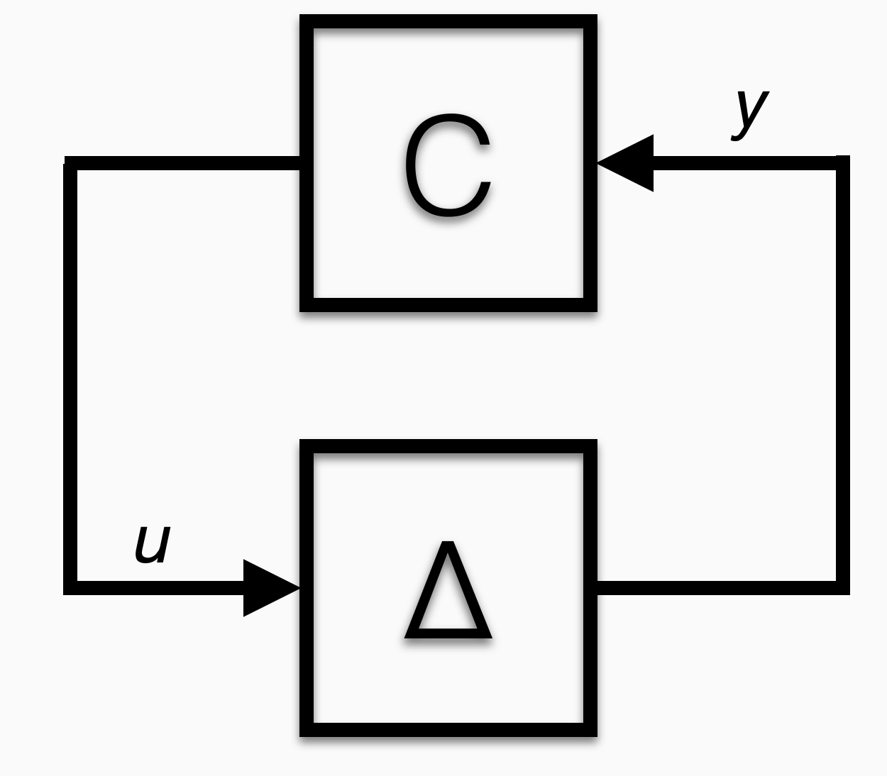
The slope bound assumption on the gradients is equivalent to assuming the black box has gain bounded between an upper and lower bound. This is the sort of thing control theorists have studied for a century. They call such nonlinear functions “sector bounded” and have a variety of tools to verify control algorithms when such uncertain nonlinearities are in the feedback loop.

In the paper “Analysis of Optimization Algorithms by Integral Quadratic Constraints,” Laurent Lessard, Andy Packard, and I translated these techniques to optimization algorithms. This let us search for Lyapunov-like proofs that your algorithm converges. With these tools, we could derive the same convergence rates and get novel robustness arguments. And the analyses were automatable, in the sense that we derived our proofs using other optimization algorithms.

A complementary approach to this problem developed by optimizers is the PEP framework, which uses a language more native to optimization. Both proof systems work because positive linear combinations of positive things are positive. Thus, you try to show a Lyapunov function decreases by writing this statement as an equality, and showing it’s the linear combination of a bunch of these inequalities. The computer can do this for you.

Lots of interesting insights come from this parallel between optimization and control. For instance, it shows there is no way to “fix” simple momentum methods like the Heavy Ball Method to prove they converge globally. The automated proof framework also helped us identify perturbations to the methods that could sometimes yield faster convergence rates or greater numerical stability.

But one thing I haven’t been able to do is turn this around: I want to teach a semester-long graduate course on PID control that would feel like my optimization class. I was hoping to get a start during this graduate seminar. I wanted to make it clear that most of the analysis could be done by Lyapunov functions. I wanted to move beyond sector-bounded nonlinear maps to more common dynamical system models in which people apply PID controllers. And I want to do all of this without ever taking a Laplace transform.

If there are any control theorists out there reading this with ideas for putting such a course together, please let me know! I know many would argue that PID controllers are solved, and the interesting stuff happens at a higher level. But to push the limits of what modern learning-control systems do, we have to understand the PID controls at the innermost loops of the complex system. Explaining this part of the architecture in a clean, modern way is a good pedagogical challenge for my control theory friends.