All Downhill From Here

Lyapunov's two methods of stability analysis

This is a live blog of Lecture 2 of my graduate seminar “Feedback, Learning, and Adaptation.” A table of contents is here.

The analysis in the last post hinted that we can use calculus to analyze the local behavior of a homeostatic system around its setpoint. I wrote up the details in these lecture notes. As long as the first terms of the Taylor series provide a reasonable approximation of the equations that define the dynamical system, we can use linear algebra to reason about how a homeostatic system maintains its steady state.

The problem with this analysis by linear proxy is that we need to somehow account for the error in the approximation. Such bookkeeping tends to be much more annoying. Determining the region of state space under which a Taylor series is accurate always amounts to frustrating calculations. These calculations also tend to be highly tuned to the particulars of the differential structure of the model. If the model slightly changes, you have to start all over again and rederive new error bounds.

To get around this sort of linear proxy analysis. Lyapunov invented an alternative method, called his second method or his direct method (I got the direct and indirect methods confused yesterday). To avoid having to create a mnemonic for what direct and indirect mean, I’m going to switch to descriptive terms for Lyapunov’s two methods: the method of linearization and the method of potential functions.

The method of potential functions is inspired by physics. The goal is to define a notion of “energy” for any possible state, and then show that energy dissipates as the dynamics unravel into the future. Mathematically, the method seeks a function that maps states to positive scalars. This function should be large far from the fixed point. It should equal zero at the fixed point and only at the fixed point. And the function should decrease along the trajectories of the dynamical system. In other words, the function must take on a lower value at time t+1 than it held at time t. Such a function is called a potential function (also often called a Lyapunov function).

You can already see that this construction should verify convergence to the fixed point. If potential decreases at every time step but is always positive, it eventually has to get to zero. The only place where the potential is zero is the fixed point. Therefore, the system has to converge to the fixed point. You can make this as rigorous as you’d like, but I find the intuition here easier than thinking about linearizations.

Proofs using potential functions are easy. Finding potential functions is hard. It’s an interesting mathematical maneuver: we have a proof technique that always works as long as you produce a particular certificate (the potential function). We thus shift the burden of proof to finding and verifying that the certificate satisfies a list of desiderata. This turns proof into a constraint satisfaction problem, one that is amenable to computer search.

Let me give a simple case in linear systems that demonstrates how this logical transformation works. We’ll do much more interesting nonlinear cases in the next class.

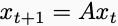
Suppose we’d like to show all trajectories of a linear dynamical system

converge to zero. From your first class on controls, you know that you can just compute the eigenvalues of A and make sure their magnitudes are all less than one. But let’s find a potential function that also certifies convergence. I need a family of functions that are positive everywhere except at the origin, where they are equal to zero. One simple family would be the strongly convex quadratics,

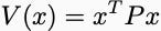
where P is a positive definite matrix with all eigenvalues greater than zero. If I want to show that the potential decreases along trajectories, I need

for all x. This is equivalent to the matrix inequality

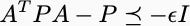
I have reduced stability analysis to solving a system of linear matrix inequalities. The set of Lyapunov functions of this form is convex. And you can use techniques from convex optimization to search for the potential function.

Now, as written so far, this seems to have turned an annoying linear algebra problem (computing eigenvalues) into an annoying convex optimization problem (semidefinite programming). Fair! But the potential function method is far more extensible. For example, suppose the system were uncertain and could evolve according to either A1 or A2 at any given time. Then you can try to find a potential function that certifies both matrices. If one exists, then the global system will be stable, even if it’s switching. The appeal of the potential function method is this sort of robustness. It lets us handle inaccurate or uncertain dynamics in ways that linearization doesn’t. In the next lecture, we’ll apply these ideas to PID controllers and draw some interesting connections between analyzing the most ubiquitous control policies and the most ubiquitous optimization methods.